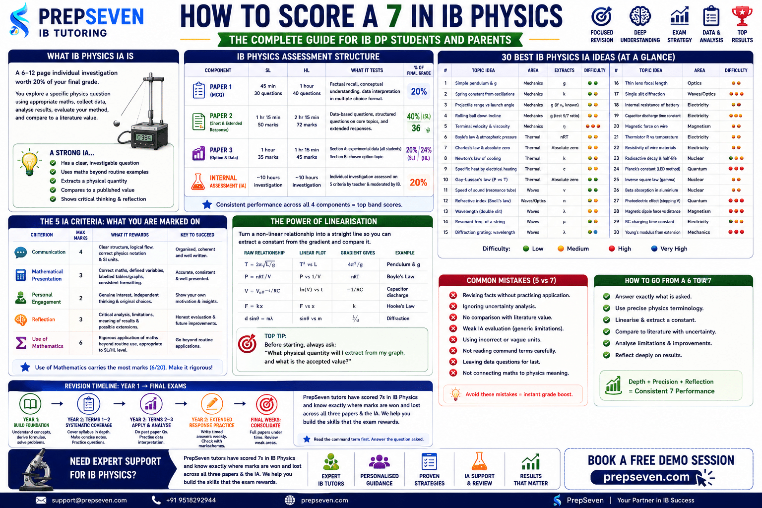
The IB Physics Internal Assessment is a 6 to 12 page individual investigation worth 20% of your final grade. Physics has a structural advantage over the other Group 4 sciences in one critical respect: almost every physical relationship between two variables is mathematically precise, which means there is almost always a published value to compare your experimental result against. This comparison, your experimentally determined value of g, or the speed of sound, or a spring constant, or a refractive index, set against the accepted value with a discussion of whether the discrepancy falls within your calculated uncertainty, is the foundation of a strong physics IA Evaluation and it is available on almost any topic you choose.
The physics investigations that score highest are those built around what you might call the linearisation structure: the research question generates a relationship between two variables, the data is linearised so that a straight-line graph can be drawn, the gradient of that graph equals a known physical quantity, and the experimental value of that quantity is extracted with uncertainty and compared to the literature value. This structure naturally satisfies the Analysis criterion, gives the Evaluation criterion something concrete to work with, and connects the investigation to syllabus content in a way that is visible throughout the write-up.
The investigations that consistently underperform are those without a physical quantity to extract, without a literature value to compare against, or without a clear relationship between the two variables that is specific enough to linearise. A student who measures how many bounces a ball makes before stopping has collected data but has no physical relationship to analyse and no published value to compare against. A student who measures how the rebound height of the same ball depends on drop height has a physically precise relationship, a linearisable graph, and a comparison point. The second topic is not more complex. It is better structured.
The single most useful question to ask about any potential physics IA topic before committing to it is: what physical quantity will I extract from the gradient or intercept of my linearised graph, and what is the accepted value of that quantity? If you can answer this question concretely before you begin collecting data, your topic has the structure it needs for strong Analysis and Evaluation. If you cannot answer it, reconsider the topic or the research question before investing time in data collection.
The Criteria Applied to Physics
Criterion
Max Marks
What Physics IAs Need
Most Common Mark Loss in Physics
Personal Engagement
2
Genuine personal motivation visible in the choice of topic or the specific physical question asked; independent choices about measurement method, variable range, or analysis approach that reflect individual thinking rather than a standard protocol
Topics chosen from recommended lists with no personal connection; investigation follows a standard textbook lab protocol exactly; Personal Engagement section describes general interest in science rather than why this specific question is interesting to this student
Exploration
6
A specific, measurable research question with the independent variable, its range, and the dependent variable with measurement method all defined; physical background at syllabus depth that explains the mechanism rather than just describing the phenomenon; all controlled variables identified with explanation of how each would affect the results if not controlled
Research question too broad to design a specific experiment; background states physical relationships without explaining their origin; controlled variables listed without explaining the direction of their effect on the results if they varied
Analysis
6
Raw data tables with absolute uncertainties on every measurement; processed data with propagated uncertainties shown step by step; graphs with best-fit lines and uncertainty bars; linearisation of the relationship where applicable; physical quantity extracted from gradient or intercept with uncertainty; units maintained throughout
No uncertainty propagation; error bars absent or not derived from the calculated uncertainty; no linearisation of a non-linear relationship; no physical quantity extracted from the graph; units dropped at intermediate steps
Evaluation
6
Percentage discrepancy between experimental and literature value calculated explicitly; assessment of whether the discrepancy falls within or beyond the experimental uncertainty; specific methodological limitations identified with their direction of effect on the measured physical quantity; realistic improvements that address each identified limitation specifically
No comparison to literature value; generic limitations (more repeats, more precise equipment) with no connection to the specific experimental setup; improvements that are unrealistic or too vague to implement; no discussion of whether the conclusion is supported by the data within its uncertainty
Communication
4
Logical structure progressing from research question through theory, method, results, analysis, and evaluation; correct physics notation including SI units and vector notation throughout; all graphs with labelled axes and units; correct significant figures throughout consistent with measurement precision; sources referenced
Missing units on axes or in tables; significant figures inconsistent with measurement precision; no clear structure distinguishing sections; physics equations written without defining symbols
The Analysis criterion in a physics IA is where the linearisation structure pays off most directly. When the relationship between your two variables is linear after transformation, you can draw a best-fit line, draw the steepest and shallowest plausible lines through the error bars to find the uncertainty range on the gradient, extract the physical quantity from the gradient with its uncertainty, and compare to the literature value. Each of these steps corresponds to marks in the Analysis criterion, and they all follow naturally from a well-chosen research question with a well-executed linearisation.
The Evaluation criterion requires the comparison to the literature value to be done properly, not just mentioned. The proper form is: calculate the percentage discrepancy between your experimental value and the literature value, compare this to the percentage uncertainty on your experimental value, and then discuss what this comparison implies. If the discrepancy is within the uncertainty, your result is consistent with the accepted value within experimental precision, and your evaluation should explain why the remaining uncertainty exists. If the discrepancy exceeds the uncertainty, there is likely a systematic error, and your evaluation should identify what it is and why it acts in the direction it does.
The Linearisation Principle: The Most Important Tool in Physics IA
Linearisation is the technique of transforming a non-linear relationship between two variables into a linear one so that a straight-line graph can be drawn, and a physical quantity can be extracted from the gradient or intercept. It is the most important analytical tool in IB Physics and the one that most clearly distinguishes a strong physics IA from a weak one.
The reason linearisation is so powerful is that a straight line has two properties that are directly useful: the gradient and the intercept. Both of these can be calculated from the graph with an uncertainty, both can be connected to known physical constants or quantities, and both can be compared to literature values. A curved graph has neither of these properties in a directly usable form.
Physical Relationship
Raw Graph
Linearised Form
Gradient Gives
Intercept Gives
Period of a simple pendulum: T = 2π√(L/g)
T vs L (curved)
T² vs L (linear)
4π²/g, allowing g to be calculated
Should be zero; non-zero intercept indicates systematic error in length measurement
Spring extension: F = kx
F vs x (linear already)
F vs x
Spring constant k directly
Should be zero; non-zero suggests pre-tension or measurement offset
Radioactive decay: N = N₀e^(−λt)
N vs t (exponential)
ln(N) vs t (linear)
Negative of decay constant −λ
ln(N₀), giving initial count rate N₀
Coulomb’s law: F = kq₁q₂/r²
F vs r (inverse square)
F vs 1/r² (linear)
kq₁q₂, allowing Coulomb’s constant to be found if charges are known
Should be zero; non-zero suggests background force or charge measurement error
Intensity and distance from point source: I = P/(4πr²)
I vs r (inverse square)
I vs 1/r² (linear)
P/4π, allowing source power to be calculated
Should be zero; non-zero suggests background intensity or offset in distance measurement
Snell’s law: n₁sin(θ₁) = n₂sin(θ₂) for fixed n₁
sin(θ₂) vs sin(θ₁) (linear)
sin(θ₂) vs sin(θ₁)
n₁/n₂, giving refractive index ratio
Should be zero; non-zero indicates systematic angle measurement error
Resonance frequency of a string: f = (1/2L)√(T/μ)
f vs 1/L (linear for fixed T, μ)
f vs 1/L
(1/2)√(T/μ), allowing wave speed or linear density to be calculated
Should be zero; non-zero indicates systematic length measurement error
Capacitor discharge: V = V₀e^(−t/RC)
V vs t (exponential)
ln(V) vs t (linear)
−1/RC, giving the time constant RC
ln(V₀), giving initial voltage V₀
Students who understand linearisation before choosing their topic will always find a better topic than students who choose first and try to fit the analysis to the data afterwards. Look at the physical relationship your research question involves, identify how to linearise it, identify what the gradient gives you, and check whether there is a published value for that quantity. If all three answers are satisfactory, the topic has the structure it needs for a strong physics IA. If any answer is unsatisfactory, either modify the question or choose a different topic.
IB Physics IA Ideas by Topic Area
The ideas below are organised by the five topic areas of the IB Physics syllabus. Each entry includes the research question format, the physical relationship being investigated, how to linearise it, what physical quantity is extracted from the gradient, and what makes the idea strong or weak across the five criteria. Every idea has been chosen because it has a clear linearisation structure and a published value to compare against.
A: Space, Time, and Motion (Mechanics)
Mechanics investigations are the most common type in IB Physics IA and include some of the most structurally clean topics available. The challenge is distinguishing between topics that have the linearisation structure and a physical quantity to extract, and those that simply measure a kinematic quantity without generating anything to compare. An investigation of how drop height affects impact velocity is less strong than one where the data allows g to be determined and compared to 9.81 m/s².
Topic Idea
Research Question
Physical Relationship
Linearisation and Gradient
Literature Value for Comparison
Simple pendulum and g
How does the length of a simple pendulum between 20 cm and 100 cm affect its period, and what value of g does the data indicate?
T = 2π√(L/g)
Plot T² vs L; gradient = 4π²/g; extract g from gradient
g = 9.81 m/s² (local value can be looked up for your latitude)
Spring constant from oscillation period
How does the mass attached to a spring between 50 g and 400 g affect the period of vertical oscillation, and what spring constant does the data indicate?
T = 2π√(m/k)
Plot T² vs m; gradient = 4π²/k; extract k from gradient and compare to k measured directly from F = kx
k from static extension measurement provides an independent comparison
Projectile range vs launch angle
How does the launch angle of a projectile between 20° and 70° affect its horizontal range, and does the data confirm the prediction from kinematic theory?
Range = v₀²sin(2θ)/g
Plot range vs sin(2θ); gradient = v₀²/g; if v₀ is measured independently, g can be extracted
g = 9.81 m/s²; maximum range at 45° is a testable prediction
Rolling ball and acceleration down a ramp
How does the angle of inclination of a ramp between 5° and 30° affect the acceleration of a rolling ball, and does the data agree with the theoretical prediction accounting for rotational inertia?
a = (5/7)g sin(θ) for a solid sphere
Plot a vs sin(θ); gradient = 5g/7; extract g and compare to accepted value; deviation from 5/7 indicates non-ideal rolling
g = 9.81 m/s²; ratio 5/7 for solid sphere is a testable prediction
Terminal velocity and viscosity
How does the radius of a ball bearing between 1 mm and 5 mm affect its terminal velocity in glycerol, and what value of viscosity does the data indicate?
v_t = 2r²(ρ-ρ_f)g / 9η (Stokes’ law)
Plot v_t vs r²; gradient = 2(ρ-ρ_f)g/9η; extract η from gradient
Published viscosity of glycerol at measured temperature (typically 1.5 Pa·s at 20°C)
The simple pendulum investigation is the most commonly submitted physics IA topic globally and the one examiners have seen most often. It is not a weak topic structurally, because it has an excellent linearisation and a precise comparison value. The risk is that it looks identical to the textbook experiment with no personal angle, which weakens Personal Engagement. Students who choose the pendulum should find a specific dimension of the investigation to make their own: investigating the effect of pendulum bob material on the period and comparing across materials with different densities, or comparing pendulum behaviour in different viscosity fluids, or using a phone accelerometer rather than a photogate to measure the period, all add a personal dimension that the standard protocol lacks.
B: The Particulate Nature of Matter (Thermal Physics)
Thermal physics investigations often involve measuring temperature changes or pressure changes as a function of a controlled variable. They are technically straightforward in most school labs and generate data that connects directly to the gas laws, heat capacity, and thermodynamic relationships in the syllabus. The challenge is finding a question with enough variable range to generate a clear trend and enough precision to extract a meaningful physical quantity.
Topic Idea
Research Question
Physical Relationship
Linearisation and Gradient
Literature Value for Comparison
Boyle’s Law verification and atmospheric pressure
How does the pressure of a trapped gas change as its volume is varied, and what value of atmospheric pressure does the PV = constant relationship indicate?
PV = nRT (at constant T); P = nRT/V
Plot P vs 1/V; gradient = nRT; if n and T are known, R can be extracted; intercept should be zero
R = 8.314 J/mol/K; atmospheric pressure at the location can be compared to weather station data
Charles’s Law and absolute zero
How does the volume of a gas change with temperature between 0°C and 100°C at constant pressure, and what value of absolute zero does the extrapolated relationship indicate?
V = nR/P × T (absolute)
Plot V vs T in Celsius; extrapolate the linear fit to find the x-intercept, which equals absolute zero in Celsius
Absolute zero = −273.15°C; the intercept of the extrapolated V-T graph should approach this value
Newton’s Law of Cooling constant
How does the rate of cooling of water depend on the temperature difference between the water and the surroundings, and what cooling constant does the data indicate?
Plot ln(T − T_ambient) vs t; gradient = −k; k characterises the specific cooling setup
Comparison of k values across different container types or insulation levels; also relates to heat transfer coefficient
Specific heat capacity by electrical heating
How does the temperature of a known mass of liquid rise with energy supplied by an immersion heater, and what specific heat capacity does the data indicate?
Q = mcΔT; E = Pt (for constant power P)
Plot ΔT vs time; gradient = P/mc; extract c from gradient with P and m known
c(water) = 4181 J/kg/K; c(ethanol) = 2440 J/kg/K; comparison to published values generates clear Evaluation
Pressure and temperature at constant volume (Gay-Lussac)
How does the pressure of a fixed volume of gas change with temperature between 0°C and 100°C, and does the data agree with the ideal gas law prediction?
P = (nR/V) × T (absolute)
Plot P vs T in Kelvin; gradient = nR/V; should be linear with zero intercept; extrapolation to P = 0 gives absolute zero
Absolute zero = 0 K; also allows verification that nR/V is consistent with known n, R, V values
C: Wave Behaviour
Wave investigations are structurally excellent for the physics IA because wave relationships are mathematically precise, physically interpretable, and directly connected to the core syllabus content. The speed of sound, the refractive index of a material, the wavelength of a light source, and the resonant frequencies of a string or air column all have published values and can be determined from the gradient of a linearised graph. Wave investigations also tend to produce clean, reproducible data in a school lab.
Topic Idea
Research Question
Physical Relationship
Linearisation and Gradient
Literature Value for Comparison
Speed of sound from resonance in a closed pipe
How does the resonant length of a closed air column change with the frequency of the tuning fork, and what speed of sound does the data indicate?
f = v/4L for first resonance (closed pipe); L = v/4f
Plot L vs 1/f; gradient = v/4; extract v from gradient
Speed of sound in air ≈ 331 + 0.6T m/s where T is temperature in Celsius; comparison to temperature-corrected value generates specific Evaluation discussion
Refractive index by Snell’s law
How does the angle of refraction of light passing from air into [glass or acrylic block] depend on the angle of incidence, and what refractive index does the data indicate?
Plot sin(θ₂) vs sin(θ₁); gradient = 1/n₂; extract n₂ from gradient
n(glass) ≈ 1.50; n(acrylic) ≈ 1.49; specific value depends on glass type and can be found from manufacturer data
Wavelength from double slit interference
How does the fringe spacing in a double slit interference pattern change with the slit separation, and what wavelength of light does the data indicate?
Δy = λD/d where D is screen distance, d is slit separation
Plot Δy vs 1/d for fixed D; gradient = λD; extract λ from gradient with D known
Wavelength of laser pointer (typically 630–680 nm for red); can be checked against manufacturer specification
Resonant frequency of a string and linear density
How does the fundamental resonant frequency of a vibrating string change with its tension, and what linear mass density does the data indicate?
f = (1/2L)√(T/μ)
Plot f² vs T; gradient = 1/(4L²μ); extract μ from gradient with L known and compare to measured μ
μ measured by weighing a known length of the string; comparison of extracted and measured μ generates specific Evaluation
Diffraction grating and wavelength determination
How does the angle of the first-order diffraction maximum from a diffraction grating change with the grating spacing, and what wavelength does the data indicate?
d sin(θ) = mλ for order m
Plot sin(θ) vs 1/d for fixed wavelength; gradient = mλ; or for fixed d plot sin(θ) vs m (integer), gradient = λ/d
Wavelength of laser or spectral line; comparison to manufacturer specification or NIST spectral data
The speed of sound from resonance in a closed pipe is one of the structurally strongest physics IA topics available at any level. It generates a T vs 1/f graph where the gradient gives v/4, it has a precise and temperature-dependent literature value that creates a specific and scientifically interesting Evaluation, and the systematic error from the end correction of the pipe (the effective length is slightly longer than the measured length) is a specific, directional, and discussable limitation that generates strong Evaluation marks. A student who measures the temperature during the experiment, corrects the literature value accordingly, and discusses how the end correction shifts all length measurements systematically in one direction has produced an Evaluation section that earns full marks.
D: Fields (Electricity, Magnetism, and Optics)
Fields investigations cover electric circuits, magnetic force, capacitors, and optics. They tend to produce highly reproducible data with clear uncertainty characteristics and, in the case of circuit investigations, are among the most accessible experiments in a school lab. The key is identifying a relationship with a physically meaningful gradient rather than simply measuring a quantity that does not connect to a known constant.
Topic Idea
Research Question
Physical Relationship
Linearisation and Gradient
Literature Value for Comparison
Internal resistance of a battery
How does the terminal voltage of a battery change as the current drawn from it is increased, and what internal resistance and EMF does the data indicate?
V = EMF − Ir (terminal voltage = EMF minus voltage drop across internal resistance)
Plot V vs I; gradient = −r (internal resistance); y-intercept = EMF
EMF can be checked with a high-resistance voltmeter; internal resistance of a standard AA cell is typically 0.1–1 Ω depending on age and type
Capacitor discharge time constant
How does the voltage across a discharging capacitor change with time, and what time constant does the data indicate for a known resistance?
V = V₀e^(−t/RC)
Plot ln(V) vs t; gradient = −1/RC; with R known, extract C and compare to labelled capacitance
Labelled capacitance on the capacitor (typically within 10–20% tolerance); also allows testing of whether capacitance is constant across discharge
Magnetic force on a current-carrying conductor
How does the force on a current-carrying wire in a magnetic field change with the current, and does the data agree with F = BIL with the known field strength?
F = BIL for a conductor of length L in field B
Plot F vs I; gradient = BL; with L measured, extract B and compare to field measured independently by Hall probe
Magnetic field of the permanent magnet measured by Hall probe or from manufacturer data
Resistance and temperature for a thermistor
How does the resistance of an NTC thermistor change with temperature between 10°C and 60°C, and does the relationship follow an exponential model?
R = R₀ e^(β/T) where T is absolute temperature and β is a material constant
Plot ln(R) vs 1/T; gradient = β; extract β and compare to manufacturer datasheet value
β values for common NTC thermistors are provided in manufacturer datasheets; typically 3000–5000 K
Focal length of a converging lens
How does the image distance change with object distance for a converging lens, and what focal length does the data indicate?
1/f = 1/u + 1/v (thin lens equation)
Plot 1/v vs 1/u; gradient = −1 (check linearity); x and y intercepts both = 1/f; extract f from intercepts
Focal length from manufacturer specification or from direct measurement at 2f; comparison across two independent methods generates strong Evaluation
E: Nuclear and Quantum Physics
Nuclear and quantum physics investigations are less common in IB Physics IAs, primarily because nuclear experiments require access to radioactive sources and detectors that not all schools have. Where they are available, they produce excellent investigations because radioactive decay is one of the most mathematically precise physical processes, with decay constants and half-lives that are known to high precision and make strong comparison values. Quantum investigations using the photoelectric effect or LED threshold wavelengths are also accessible in well-equipped schools.
Topic Idea
Research Question
Physical Relationship
Linearisation and Gradient
Literature Value for Comparison
Radioactive decay constant and half-life
How does the count rate of a radioactive source change with time, and what half-life does the data indicate?
N = N₀e^(−λt); activity A = A₀e^(−λt)
Plot ln(A) vs t; gradient = −λ; extract half-life as t₁/₂ = ln(2)/λ
Published half-life values from NIST or IAEA nuclear data; Ba-137m (half-life 2.55 minutes) and Am-241 (half-life 432 years) are common school sources
Planck’s constant from LED threshold voltage
How does the minimum voltage required to cause a light-emitting diode to emit light vary with the wavelength of light it emits, and what value of Planck’s constant does the data indicate?
eV_threshold = hf = hc/λ; V_threshold = hc/(eλ)
Plot V_threshold vs 1/λ for multiple coloured LEDs; gradient = hc/e; extract h from gradient with c and e known
h = 6.626 × 10⁻³⁴ J·s; comparison of experimental to accepted Planck’s constant generates a direct test of the photon model
Inverse square law for gamma radiation
How does the count rate from a gamma source change with distance, and does it follow the inverse square law for a point source?
I = k/r² for a point source in the absence of absorption
Plot count rate vs 1/r²; should be linear through origin if inverse square law holds; non-linearity indicates absorption or geometry effects
The inverse square law itself is the prediction; deviations from linearity are physically interesting and provide Evaluation material
Absorption of beta radiation by aluminium
How does the count rate of beta radiation from [source] change with the thickness of aluminium absorber, and what absorption coefficient does the data indicate?
I = I₀e^(−μx) where μ is the linear attenuation coefficient
Plot ln(count rate) vs thickness; gradient = −μ; extract μ and compare to published values for beta attenuation in aluminium
Published attenuation coefficients for beta radiation in aluminium are available from NIST radiation data tables
Photoelectric effect: stopping voltage vs frequency
How does the stopping voltage required to prevent photocurrent in a photoelectric experiment vary with the frequency of incident light, and what value of Planck’s constant does the data indicate?
eV_stop = hf − φ where φ is the work function
Plot V_stop vs f; gradient = h/e; extract h from gradient with e known; x-intercept = φ/h (threshold frequency)
h = 6.626 × 10⁻³⁴ J·s; threshold frequency can be compared to published work function for the metal used
Planck’s constant from LED threshold voltages is one of the most conceptually satisfying physics IA topics because it recreates, with basic school equipment, one of the most important experiments in the history of quantum physics. The investigation requires measuring the threshold voltage for LEDs of several different colours, plotting V_threshold against 1/λ, and extracting h from the gradient. The comparison of the experimental Planck’s constant to the accepted value of 6.626 × 10⁻³⁴ J·s is both meaningful and direct. Personal Engagement is strong because the investigation is a genuine test of the photon model rather than a verification of an already-familiar relationship, and the connection to the photoelectric effect and the development of quantum theory provides rich background material.
Topics That Consistently Underperform and Why
Overused or Weak Topic
Why It Underperforms
What to Do Instead
How does drop height affect the rebound height of a ball?
No physically precise relationship to extract. The coefficient of restitution can be calculated, but it is not a quantity with a precise literature value, and the investigation generates no linearisable graph. Evaluation is limited to generic comments about energy loss.
Investigate how the coefficient of restitution depends on temperature, or how it varies across balls of different material at fixed conditions. This adds a genuine independent variable and allows the energy loss mechanism to be discussed in terms of material properties.
How does the length of a wire affect its resistance?
Structurally this is fine: R vs L is linear with gradient ρ/A. But it is one of the most submitted IA topics globally and the standard school electricity lab. Without a personal angle it has no Personal Engagement, and the Evaluation limitations are entirely generic.
Investigate how resistivity varies with temperature for a specific conductor, or compare resistivity across different wire materials. The resistivity extracted from the gradient has a precise literature value for each material, and temperature dependence generates richer Evaluation.
How does temperature affect the resistance of a wire?
Similar to above: the relationship exists but without a specific physical quantity extracted from the linearised graph, the Analysis stays at the descriptive level. Students often plot R vs T without recognising that ln(R) vs 1/T for a thermistor, or R vs T for a metallic conductor, each give a physically meaningful gradient.
Specify the type of conductor explicitly. For a thermistor, extract the β parameter from the ln(R) vs 1/T graph and compare to the manufacturer datasheet. For a metal wire, extract the temperature coefficient of resistivity and compare to published values.
How does the angle of a ramp affect the time taken for a ball to roll down?
Measuring time by stopwatch introduces large random uncertainty. The relationship between angle and time is not directly linearisable. No precise physical quantity is extracted and there is nothing to compare the result against.
Use the same ramp but measure acceleration using video analysis or motion sensors. Plot acceleration vs sin(θ); gradient = (5/7)g for a solid sphere; extract g and compare to 9.81 m/s². This transforms an unfocused topic into a structurally strong IA.
How does the number of coils in an electromagnet affect its lifting force?
The relationship between number of coils and magnetic force is not straightforward because it depends on the geometry, the core material, and saturation effects that are not predictable from simple theory. No precise literature value exists for comparison, and the Evaluation cannot go beyond generic comments about magnetic saturation.
Investigate how the force between two magnets depends on their separation, using F vs 1/r³ for a dipole-dipole interaction. This generates a linearisable graph with a gradient connected to the magnetic moment of the magnets, and deviations from the dipole model at short distances generate substantive Evaluation.
Uncertainty Analysis in Physics IAs: The Full Chain
Uncertainty analysis in IB Physics is not a box-ticking exercise. It is a connected chain from raw measurement precision through to the final comparison with a literature value, and every link in the chain needs to be present and consistent for the Analysis and Evaluation criteria to score highly. Many students perform parts of the chain correctly but break the connection somewhere, producing an uncertainty analysis that looks complete but is internally inconsistent.
Step in the Chain
What It Involves
Common Error That Breaks the Chain
Raw measurement uncertainty
Record the absolute uncertainty on every raw measurement based on the instrument precision. For analogue instruments this is half the smallest division. For digital instruments it is typically the last significant figure.
Recording data without uncertainties, or stating uncertainties inconsistently (e.g. ±0.5 mm for some readings and ±1 mm for others from the same ruler)
Processed data uncertainty (propagation)
Propagate uncertainties through calculations: add absolute uncertainties for sums and differences; add percentage uncertainties for products and quotients; multiply percentage uncertainty by the power for exponential relationships.
Propagating by adding absolute uncertainties for all operations regardless of whether they are additive or multiplicative; ignoring propagation entirely and only reporting raw uncertainties
Error bars on the graph
Plot error bars on each data point with size equal to the propagated uncertainty on the processed y-value and the absolute uncertainty on the x-value.
Drawing error bars without basing their size on the calculated propagated uncertainty; omitting error bars entirely; drawing all error bars the same size regardless of the calculated variation
Gradient uncertainty from the graph
Draw the best-fit line, then draw the steepest and shallowest plausible lines through the error bars. Calculate the gradient of each and take the range as the uncertainty on the gradient.
Calculating gradient uncertainty by propagating the uncertainties on individual data points rather than from the range of plausible gradients; omitting gradient uncertainty entirely
Physical quantity uncertainty from gradient
Propagate the gradient uncertainty through to the physical quantity extracted from it. For example if g = 4π²/gradient, the percentage uncertainty on g equals the percentage uncertainty on the gradient.
Reporting the extracted physical quantity without an uncertainty; not connecting the gradient uncertainty to the uncertainty on the physical quantity
Comparison to literature value
Calculate the percentage discrepancy between your experimental value and the literature value. Compare this to your percentage uncertainty. Discuss whether the discrepancy is within uncertainty (random error only) or beyond uncertainty (systematic error present).
Not calculating a percentage discrepancy at all; calculating it but not comparing it to the experimental uncertainty; concluding that the experiment was successful without this comparison
The most common place where the chain breaks is between the error bars on the graph and the gradient uncertainty. Students who draw error bars correctly but then calculate the gradient from the coordinates of two data points rather than from the range of plausible lines through the error bars have disconnected the uncertainty analysis from the graph. The gradient uncertainty must come from the graph, specifically from the range of gradients that are consistent with the error bars, not from the uncertainty on individual data points.
Quick Reference: 30 IB Physics IA Ideas
Topic
Topic Area
Physical Quantity Extracted
Linearisation
Difficulty
Simple pendulum and g
Mechanics
g = 4π²/gradient of T² vs L
T² vs L
Low
Spring constant from oscillation
Mechanics
k = 4π²/gradient of T² vs m
T² vs m
Low
Projectile range vs launch angle
Mechanics
g from gradient if v₀ known
Range vs sin(2θ)
Medium
Rolling ball acceleration down ramp
Mechanics
g from gradient; test 5/7 ratio
a vs sin(θ)
Medium
Terminal velocity and viscosity (Stokes’ law)
Mechanics
Viscosity η from gradient
v_t vs r²
Medium-High
Boyle’s law and atmospheric pressure
Thermal
nRT from gradient
P vs 1/V
Low-Medium
Charles’s law and absolute zero
Thermal
Absolute zero from x-intercept
V vs T (Celsius)
Low-Medium
Newton’s law of cooling constant
Thermal
Cooling constant k from gradient
ln(T − T_amb) vs t
Medium
Specific heat capacity by electrical heating
Thermal
c from gradient P/mc
ΔT vs time
Low-Medium
Gay-Lussac’s law and absolute zero
Thermal
Absolute zero from P vs T extrapolation
P vs T (Kelvin)
Low-Medium
Speed of sound from closed pipe resonance
Waves
Speed of sound from gradient
L vs 1/f
Medium
Refractive index by Snell’s law
Waves/Optics
n₂ from gradient
sin(θ₂) vs sin(θ₁)
Low-Medium
Wavelength from double slit interference
Waves
λ from gradient with D known
Δy vs 1/d
Medium
Resonant frequency of a string
Waves
μ from gradient
f² vs T
Medium
Diffraction grating wavelength determination
Waves
λ from gradient d·sin(θ)/m
sin(θ) vs m
Medium
Thin lens focal length
Optics
f from x and y intercepts of 1/v vs 1/u
1/v vs 1/u
Low-Medium
Wavelength from single slit diffraction
Waves
λ from minima positions vs slit width
sin(θ_min) vs m
Medium-High
Internal resistance of a battery
Fields/Electricity
r and EMF from gradient and intercept
V vs I
Low
Capacitor discharge time constant
Fields/Electricity
RC and C from gradient
ln(V) vs t
Medium
Magnetic force on current-carrying wire
Fields/Magnetism
B from gradient with L known
F vs I
Medium
Thermistor resistance vs temperature
Fields/Electricity
β from gradient
ln(R) vs 1/T
Medium
Resistivity of different wire materials
Fields/Electricity
ρ from gradient with A known
R vs L
Low
Radioactive decay constant and half-life
Nuclear
λ and t₁/₂ from gradient
ln(A) vs t
Medium
Planck’s constant from LED threshold voltage
Quantum
h from gradient with c and e known
V_threshold vs 1/λ
Medium-High
Inverse square law for gamma radiation
Nuclear
Tests inverse square law directly
Count rate vs 1/r²
Medium
Beta radiation absorption in aluminium
Nuclear
μ from gradient
ln(count rate) vs thickness
Medium
Photoelectric effect stopping voltage
Quantum
h from gradient; threshold from intercept
V_stop vs f
High
Magnetic dipole force vs separation
Fields/Magnetism
Tests dipole model; extracts magnetic moment
F vs 1/r³
High
RC circuit charging time constant
Fields/Electricity
RC from gradient; compare to R×C calculated
ln(V_max − V) vs t
Medium
Young’s modulus from wire extension
Mechanics
Young’s modulus E from gradient
Stress vs strain (F/A vs ΔL/L)
Medium-High
Need help developing your IB Physics IA?
PrepSeven tutors have guided students to top IA scores across all areas of IB Physics. We help you build the linearisation structure, execute the uncertainty chain correctly, and write an Evaluation that compares your result to a literature value with the specificity that earns full marks.